Dr. Ioan Valeriu Grossu
University of Bucharest, Faculty of Physics, Romania http://www.fizica.unibuc.ro/fizica/main.asp
ABSTRACT
C# object oriented engine for simulating 3D relativistic many-body systems with covariant bi-particle force. It was developed for .Net Framework 4.8 in Microsoft Visual Studio 2022.
Second order Runge-Kutta algorithm
Reactions Engine, tested on Relativistic Nuclear Collisions at both 4.5 A GeV/c (DUBNA/SKM200 Collaboration) and 200 A GeV/c (maximum BNL energy)
High Precision Module (tested on 50 decimals for analyzing the Gravitational Butterfly Effect in Relativistic Nuclear Collisions)
Support for massless particles
QCD confinement algorithm tested on proton-proton collisions at sqrt(s) = 10 GeV
Retarded interactions algorithm tested on a 2-Body gravitational-like system
Implementtion of time reversal precision test, and various chaos analysis specific instruments
Flexible OOP solution developed in agreement with SOLID principles.
The system evolution is saved into, easy to use, comma separated values files (recognized also by Microsoft Excel)
Implementation of more than 100 unit tests
XCOPY deployment strategy
RELEASE NOTES
Chaos Many-Body v09.1.5
Migration from .Net Framework 4.7.1 to .Net Framework 4.8
Covariant treatment of bi-particle force
Reaction module improvements
Example of use: relativistic nuclear collisions at FAIR energies
Chaos Many-Body v08.1
Migration from .Net Framework 4.0 to .Net Framework 4.7.1
Implementation of a clustering algorithm for Pentaquark identification
Chaos Many-Body v08 (Quark Version)
Simulations\Quark Collision: quark toy-model for proton-proton collisions at sqrt(s) = 10GeV
Simulations\Retarded Interaction: gravitational-like 2-Body system with retarded interactions
Code refactoring to SOLID
Unit tests project
The csv simulation output files are not backward compatible!
Chaos Many-Body v07
Not published
Chaos Many-Body v06
Support for massless particles
Simulations\Collider: added some specific reactions with photons
High Precision\Micro Black Hole: example of a bound quantum system composed by 2 massless particles with gravitational force
Help\Options: application options (e.g. High precision maximum number of decimals)
Chaos Many-Body v05
Implementation of the Mean Free Time, defined as the mean time between two collisions resulting in a stimulated decay. It can be introduced as a parameter in the XML reactions file and, as opposed to the particle lifetime, is measured in the observation system.
Analysis\Chaos Analysis\Double\Other: Fuzzy algorithm for probability distributions.
Analysis\Relativistic Formulas XLS: Implementation of new functionalities.
Math\Vector\GetRandomVector: Bug correction
Simulations\Collider: New example of use for relativistic nuclear collisions at 200 A GeV/c (maximum BNL energy)
Chaos Many-Body v04.2
Analysis\Chaos Analysis\Decimal: Implementation of a decimal (base 10 number representation) version of the Chaos Analysis tools
Analysis\Chaos Analysis\...\Other Tab: Computes the probability distribution for the data stored in one specified csv file column
Analysis\Chaos Analysis\...\Compare Tab: Implementation of phases space distance between two N-Body systems, as a function of time
Analysis\Relativistic Formulas XLS: Opens an excel template containing usual relativistic formulas for facilitating processing of Monte Carlo log files (Microsoft Excel is a requirement for this functionality)
High Precision\Gravity: New example of use: Simplified nuclear relativistic collisions toy-model for analyzing the gravitational Butterfly Effect in relativistic nuclear collisions
Simulations\Cumulative Effect: New example of use: relativistic nuclear collisions for targets containing one pr more alpha particle(s)
Chaos Many-Body v04
High Precision Many-Body Engine
Example of use: study on the Butterfly Effect of the gravitational force in a relativistic nuclear collision toy-model (46 digits precision used)
Chaos Many-Body v04.1
By default, both a + b -> c + d, and a + b -> d + c reactions are allowed. For enforcing only the a + b -> c + d channel, set the CanSwitch tag to false in the reactions XML file.
Analysis\Chaos Analysis\...: "Average Y" new measure for the average of f(x) with respect to x variable
Bug Fix: in the particularly case of two identical particles head-on collision with collider mechanism, reactions were not treated.
Chaos Many-Body v03
Migration from .Net Framework 2.0 to .Net Framework 4.0
Implementation of: Structural Lyapunov Exponent
Reverse simulation precision test (only for systems without reactions, and non-parallel simulations!)
Chaos Many-Body v02
Possibility to dynamically add particle properties (spin, isospin etc.)
Time calculated in particle's reference frame, according to the successive values of instantaneous velocity
Reactions: a + b -> c + d, a -> b + c (decays), and stimulated decays
More complex schemas could be implemented by considering "virtual" particles with zero lifetime
Example: for the reaction a + b -> c + d + e one can consider f -> d + e. The engine will process the following sequence: a + b -> c + f; f -> d + e
Implementation of: Global Lyapunov Exponent, and Clusterization Maps
Basic support for Monte-Carlo simulations
Nuclear relativistic collisions example of use
Chaos Many-Body v01
Implementation of: Lyapunov Exponent, Fragmentation Level, Relativistic Virial Coefficient, and Average System Radius
Energy conservation precision test
INSTALLATION
Prerequisites: Microsoft .NET Framework 4.7.1
XCopy deployment strategy (simply copy/paste the folder containing the application)
EXAMPLE OF USE
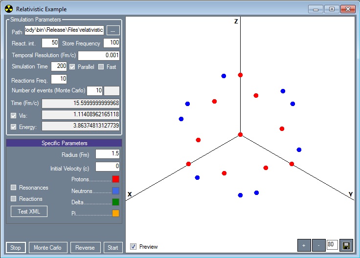
In the Applications directory, double click on the ManyBody.exe file. In the Chaos Many-Body Engine v.x screen, select Simulations\Relativistic. The following screen will be displayed.
|
In the "Simulation Parameters" section of each example (Harmonic, Relativistic, Collision etc.), you can specify values for the simulation specific parameters:
- The path for the output files;
- Setting an appropriate value for the "Reactivity interval" parameter could significantly contribute to the performance. However, a high value could freeze the application during the simulation process;
- A high value for the "Store frequency" parameter will affect only the save time interval, but not the simulation precision. A small value for it will result in creating huge output files;
- You can specify also the integration interval ("temporal resolution") and the simulation time;
- For systems with reactions you can specify the reactions check frequency (a low value could significantly affect the performance). However, for a better precision, the application will automatically increase this frequency under certain circumstances;
- Usually, we simultaneously simulate two identical systems with slightly different initial conditions, in order to analyze the Butterfly Effect. By checking the "Parallel" checkbox, each Many-Body system will be computed on a separate thread;
- Check the "Fast" checkbox in order to use a fast version of the second order Runge-Kutta algorithm (the precision could be lower);
- Uncheck the "Energy conservation test" if you do not want to perform a precision test;
- The time and the virial coefficient ("Vis") are also displayed.
Press "Start" for simulating a single event.
For simulating a set of events, specify the number of events parameter, and press "Start Monte Carlo".
The simulation ends after the specified simulation time, or by pressing "Stop".
For a Reverse Simulation Precision Test, press the Reverse button. This test does not apply for:
- Systems with reactions
- Parallel simulations
- Monte Carlo simulations
Basic analysis of simulations output
Select from menu: Analysis\Chaos Analysis\Double (for base 2 numbers - double .Net variables), or Analysis\Chaos Analysis\Decimal (for base 10 numbers - decimal .Net variables)
Note: The Chaos Analysis - Decimal version (not available any more starting with CMBE v08) is recommended for analyzing the high precision simulations output files
Note: Each simulation process could refer to one or more many-body systems. Most commonly, we simulate two identical systems with slightly different initial conditions (study of butterfly effect). For each many-body system there are two output csv files: the header (containing the list of all initial and generated particles, with the corresponding creation time information), and the data file, which contains information on the system evolution in time (position and momentum of every constituent). The files conform to the following naming rule: {File Name}.{Type}.{The Many-Body System Index}.csv, where {Type} could be hdr (for the header file), or dat (for the data file).
Press the "Open" button and choose one of the files corresponding to the Many-Body system of interest (it does not matter if you choose the hdr or the dat file)
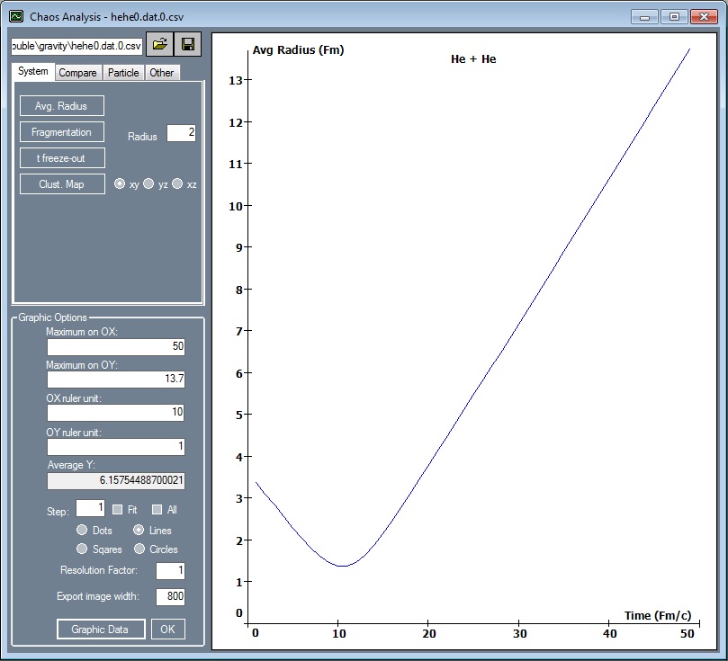
In the System tab, you can access: the fragmentation level (with the interaction radius as parameter), the average system radius represented as a function of time, the "Clusterization Map", and the freeze-out time.
|
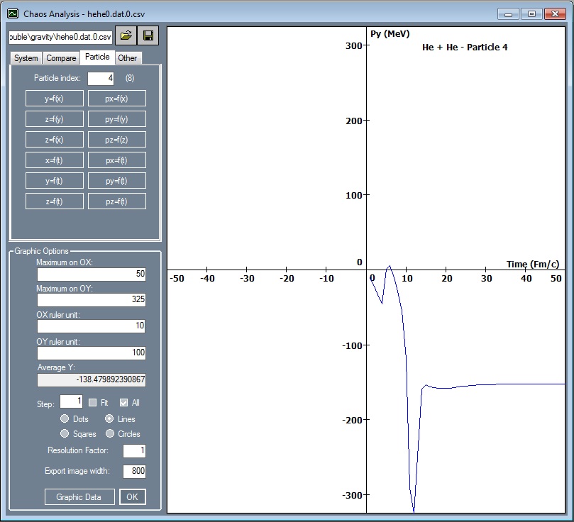
In the Particle tab, you can analyze different parameters for each individual constituent of the system (the constituent index can be specified as parameter in the "Particle index" textbox)
|
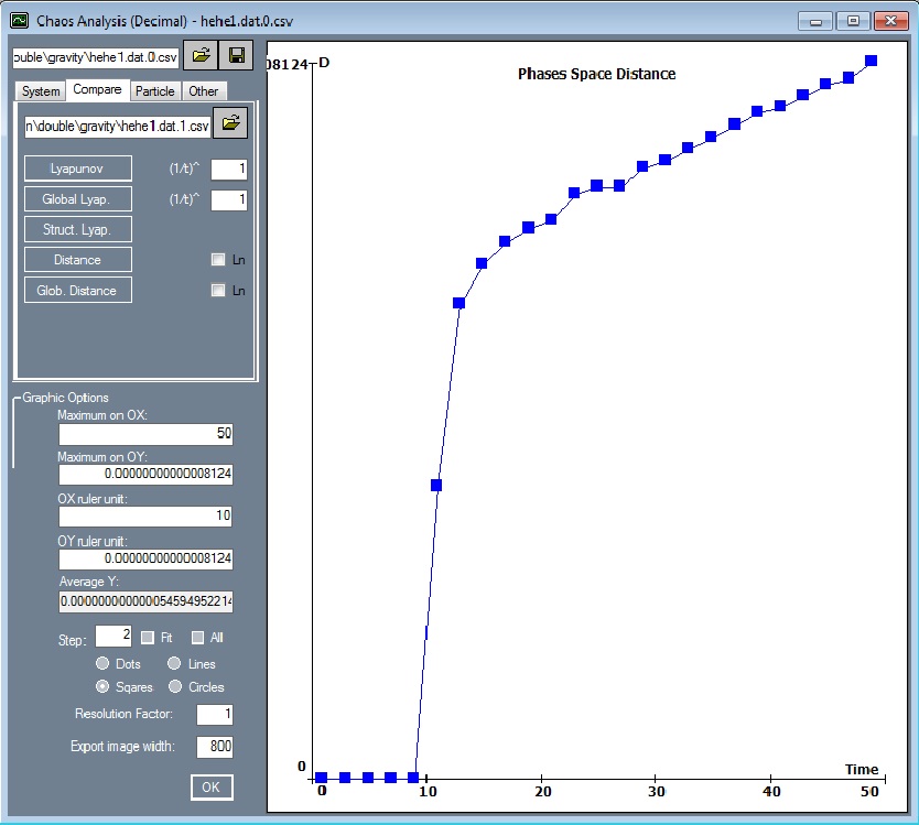
In the Compare tab, you can access: the Lyapunov Exponent (specify the power of 1/t as parameter), the Global Lyapunov Exponent, the Structural Lyapunov Exponent, the Phase Space Distance, and the Global Phase Space Distance as functions of time
|
Most commonly, we implemented each simulation as a set of two identical many-body systems with slightly different initial conditions (butterfly effect). As previously mentioned, the corresponding output files will be named: {File Name}.{Type}.0.csv and, respectively, {File Name}.{Type}.1.csv. Thus, we can use these files for estimating the Lyapunov exponent.
It is important to notice that, as the structure of two systems can significantly change in time, the multi-dimensional Lyapunov exponent cannot be applied to systems with reactions. In this case we considered the "Global Lyapunov Exponent", which is based on the resultant position vector, and the resultant momentum vector, corresponding to each many-body system.
In the "Graphic Options" section it is possible to change the appearance of any graphical representations
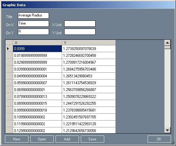
The "Graphic Data" button can be used for accessing the data used for the current graphical representation. The information can be opened/saved from/in XML files. One can also manually introduce data for a new graphical representation.
|
Basic processing of Monte Carlo simulations output
Select Analysis\Tools from menu
Open any data file member of a Monte Carlo simulation.
It is possible to process all events, or only the events between Index start and Index end.
A particle is considered free, if the distance to any other constituent from the system is grater than the Distance parameter.
You can get only the free particles, only clusters or, all information.
Check the Time Evolution check box for obtaining the desired information, for each event, and for every moment of time. Uncheck it, for obtaining only the final state of each event.
You can select all particles types (the Filter particles parameter), or only the list of desired types (e.g. specify P,N in order to select only protons and neutrons).
Check the Add header info checkbox for adding, for each event, a header line containing the event number and its corresponding number of lines.
A tool for converting csv to positional text files is also provided.
Select Analysis\Simulation Log Analysis from menu
Open a Monte Carlo simulation log file
The Log Data section is displaying the data contained in the log file, together with some calculated columns (e.g. momentum)
The Log Summary section is displaying aggregated data for each simulation from the log file (e.g. particles count)
The Entropy button is used for calculating the phase-space entropy corresponding to the entire file (all simulations from the log)
The Structural Entropy button is used for calculating the structural entropy (based only on particle types) corresponding to the entire file (all simulations from the log)
Application to a classical three-body problem with harmonic potential
Select Simulations\Harmonic from menu (or High Precision\Harmonic for the similar high precision simulation)
We present the simulation of a classical system with harmonic potential, composed by three material points placed initially at rest, in the vertices of an arbitrary triangle.
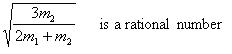
By considering m1=m3, one can notice that the constituent trajectories are closed only when the following condition is satisfied (Lissajous-like equation):
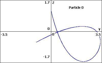
m1=m3=1, m2=6 - The Lissajous-like condition is satisfied |
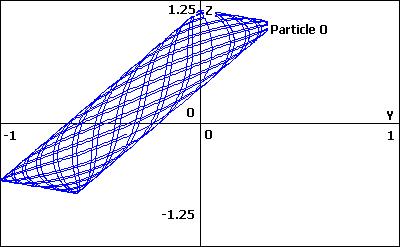
m1=m3=6, m2=1 - The Lissajous-like condition is not satisfied |
Application to a nuclear toy-model
Select Simulations\Relativistic from menu
We present the simulation of a relativistic nuclear system, composed by 21 nucleons initially placed in the vertices of a centered, regular dodecahedron, and with radial initial velocities. The bi-particle interaction is described by a Yukawa potential, together with a coulombian term.
The initial radial velocity and the initial dodecahedron radius can be specified as parameters (more parameters can be modified by accessing the corresponding code [AppPath]\ManyBody\Simulations\SimulationRelativisticExample.cs).
In function of the initial velocity parameter, one can notice the existence of three regions:
a) the oscillation regime (only a few constituents can escape from the system, unitary virial coefficient, fragmentation level closed to zero)
b) an intermediary region, characterized by a partial degree of fragmentation, which could be intuitively connected with the nuclear fragmentation mechanism
c) the expansion regime (the system is decomposed into its elementary constituents, the degree of fragmentation reaches the maximum value)
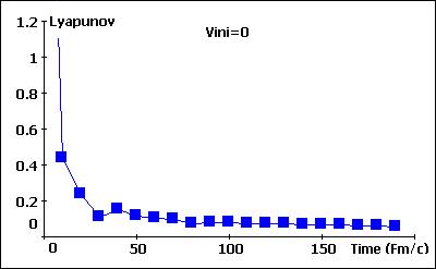
The Lyapunov Exponent for Vini=0 |
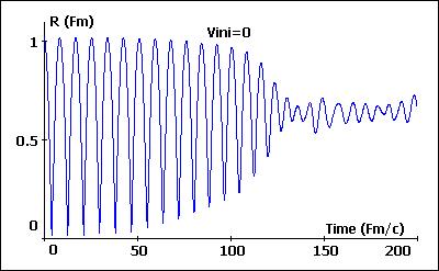
The average system radius as a function of time, for Vini=0 |
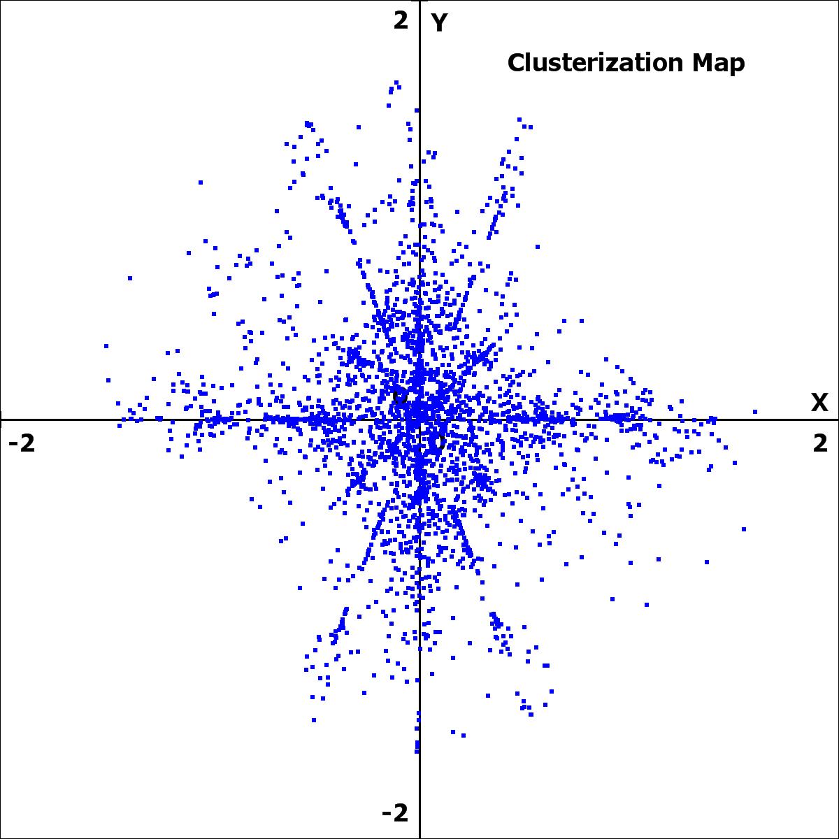
The Clusterization Map for Vini=0 |
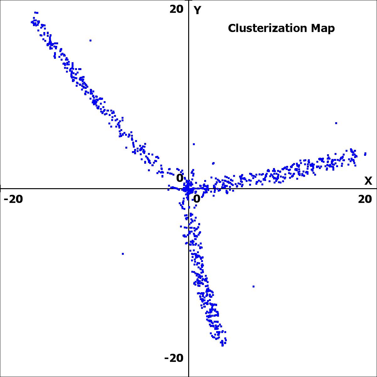
The Clusterization Map for Vini=0.5 |
Check the "Reactions" check-box to enable the reactions engine. As an example, we considered:
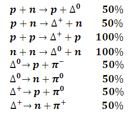
One can simply change the \\Docs\Reactions.xml file in order to add the specific reactions of interest. The "Test XML" button demontsrates how a reactions xml file can be programmatically generated.
Relativistic nuclear collisions example
Select Simulations\Collision from menu (or High Precision\Collision for the similar high precision simulation)
The momentum per nucleon can be specified as parameter.
Use the Collider checkbox in order to switch between collider and projectile/target modes.
Use the Reactions checkbox for enable/disable the reactions engine. You can simply change the \\Docs\Reactions.xml file in order to consider the specific reactions of interest.
The collision parameter can be specified as parameter, or can be randomly generated.
Choose the projectile and the target nucleus (H, Li, He, C, O, Cu, Au) from the appropriate section.
The free particles in final state, for each Monte Carlo event, are stored in the [FileName].log.csv file.
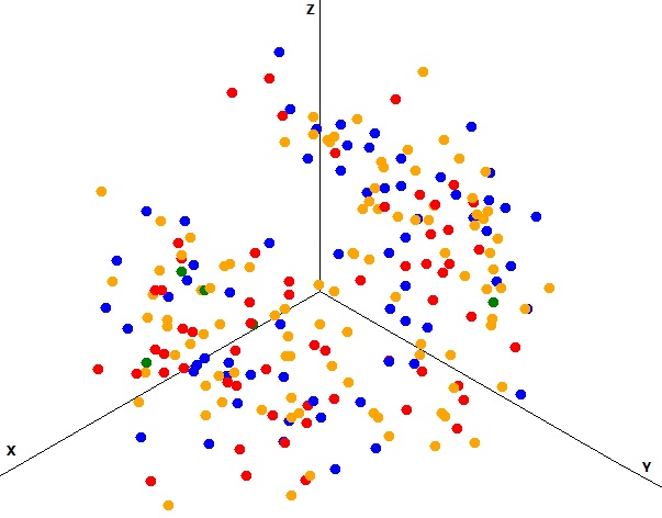
Cu + Cu at 4.5 A GeV/c - collider (p - red, n - blue, pi - yellow, delta - green) |
Relativistic nuclear collisions at 200 A GeV/c (maximum BNL energy)
Select Simulations\Collider from menu.
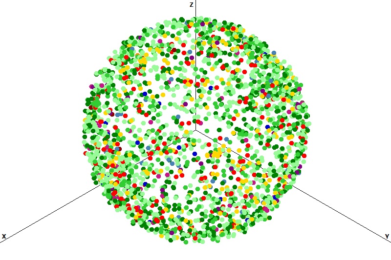
Au + Au at 200 A GeV/c, collider mechanism, b = 0 |
Proton-Proton collisions at sqrt(s)=10GeV
Select Simulations\Quark Collision from menu.
For Pentaquark multiplicity see the quark.pentaquark.log.csv file, generated into the Monte-Carlo simulation output folder (the file is generated only if there is at least one Pentaquark event)
Retarded interactions example of use
Select Simulations\Retarded Interaction from menu.
UNIT TESTS
For unit tests see the ManyBody.Test.csproj project
CODE EXAMPLE
The windows forms application (ManyBody.exe) provided together with the engine (Engine.dll, Data.dll, Math.dll) could be considered as an example of use. The "SimulationHarmonicExample", "SimulationRelativisticExample", "SimulationCollisionExample" etc. classes (\\Sources\ManyBody\Simulations\) extend the SimulationBase class, and demonstrate how the engine could be used for implementing the specific many-body system of interest.